MATH 533 | Course Introduction and Application Information - Applied Mathematics and Statistics – With Thesis

Course Name

Numerical Methods for Ordinary Differential Equations using Programming Languages

Code	Semester	Theory (hour/week)	Application/Lab (hour/week)	Local Credits	ECTS
MATH 533	Fall/Spring	3	0	3	7.5

Prerequisites	None
Course Language	English
Course Type	Elective
Course Level	Second Cycle
Mode of Delivery	-
Teaching Methods and Techniques of the Course	Lecture / Presentation
National Occupation Classification	-
Course Coordinator	Doç. Dr. Sevin GÜMGÜM
Course Lecturer(s)	Doç. Dr. Sevin GÜMGÜM
Assistant(s)	Arş.Gör. Merve KAHRAMAN ARİMAN

Course Objectives	The aim of this course is to provide a theoretical and practical foundation for the numerical solution of ordinary differential equations, enabling students to understand the concepts of convergence, stability, and error analysis, and to develop effective algorithms for Runge–Kutta and multistep methods, stiff system solvers, adaptive step-size control, and basic boundary value problems; within this scope, the course aims to equip students with the ability to implement and interpret numerical solvers using MATLAB, Mathematica, or Python.
Learning Outcomes	The students who succeeded in this course; Analyze the convergence, stability, and accuracy properties of numerical ODE solvers. Derive advanced single-step and multi-step methods. Apply techniques for handling stiff differential equations, including implicit methods. Assess the suitability of numerical methods for specific ODE problems. Solve boundary value problems using shooting, finite difference, and collocation methods. Implement numerical ODE algorithms in programming languages.
Course Description	This course introduces the fundamental concepts of error, stability, and convergence in ordinary differential equations (ODEs). Students will learn to implement and analyze numerical methods for both initial and boundary value problems, gaining hands-on experience with computational tools through programming-based assignments, projects, and in-class demonstrations. The course teaches how good programming practices affect the speed and accuracy of numerical solvers.
Related Sustainable Development Goals

Course Category	Core Courses
	Major Area Courses
	Supportive Courses
	Media and Management Skills Courses
	Transferable Skill Courses

Week	Subjects	Related Preparation
1	Review and Foundations: Review of ODEs: existence, uniqueness, well-posedness, Types of errors: truncation, round-off. Floating-point arithmetic, Brief review of basic methods: Euler, Taylor series methods, Order of accuracy, local and global error.	Griffiths & Higham (Ch 1-2).
2	Advanced Runge-Kutta (RK) Methods I (Explicit): Derivation of general explicit RK methods, Order conditions, Higher-order explicit RK methods , Error estimation for RK methods, embedded RK pairs Programming focus: Implementing RK4 and higher-order explicit RK methods; writing general RK solvers; embedded RK error estimators.	Griffiths & Higham (Ch 3.1-3.4).
3	Advanced Runge-Kutta (RK) Methods II (Implicit): Implicit RK methods: Gauss, Radau, Lobatto methods, Collocation methods for IVPs and their connection to implicit RK, Computational challenges of implicit methods	Griffiths & Higham (Ch 3.5, 3.6).
4	Linear Multistep Methods I: General form of LMMs: explicit (Adams-Bashforth) and implicit (Adams-Moulton), Derivation from polynomial interpolation/numerical integration, Order of accuracy. Programming focus: Implementing Adams-Bashforth and Adams-Moulton integrators using modular code structures.	Griffiths & Higham (Ch 4.1-4.2).
5	Linear Multistep Methods II & Predictor-Corrector Methods: Zero-stability, Root condition, Dahlquist's theorems, Predictor-Corrector schemes, local error estimation for P-C, Variable step-size LMMs. Programming focus: Writing adaptive predictor–corrector solvers; variable step-size implementation.	Griffiths & Higham (Ch 4.3-4.5).
6	Absolute Stability and Stiff ODEs I: Absolute stability: regions of absolute stability for RK and LMMs, Graphical interpretation of stability regions, Introduction to stiff ODEs: Definition, characteristics, stiffness ratio.	Griffiths & Higham (Ch 5.1-5.3).
7	Stiff ODEs II: Implicit Methods for Stiff Problems: A-stability, L-stability, stiff-stability, Backward Differentiation Formulas (BDFs): derivation, properties, stability regions, Implementation details: Newton's method for implicit equations, Jacobian approximation. Programming focus: Visualizing stability regions numerically, coding the BDF family	Griffiths & Higham (Ch 5.4-5.6).
8	Adaptive Step-Size Control: Error estimation for explicit RK methods, Error estimation for LMMs Control strategies: PI controllers, step-doubling, step-halving.	Griffiths & Higham (Ch 6).
9	Adaptive Step-Size Control: Error estimation for explicit RK methods, Error estimation for LMMs Control strategies: PI controllers, step-doubling, step-halving.	Griffiths & Higham (Ch 6)
10	Boundary Value Problems I: Review of Shooting Methods, multiple shooting, Limitations and advantages of shooting methods, Connection to solving systems of nonlinear algebraic equations. Programming focus: Implementing single/multiple shooting	Sauer, Chapters 7
11	Boundary Value Problems II: Finite Difference Methods:Finite Difference approximations for derivatives,Formulation of finite difference schemes for linear BVPs, Consistency, stability, and convergence of FDM for BVPs, Finite Difference methods for nonlinear BVPs	Sauer, Chapters 7
12	Boundary Value Problems III: Collocation Methods, Introduction to Collocation Methods for BVPs, Choice of basis functions, Choice of collocation points, Formulation for linear and nonlinear BVPs, Comparison with finite difference methods.	Instructor provided notes/papers
13	Project Presentations
14	Project Presentations
15	Semester Review
16	Final Exam

Course Notes/Textbooks

Griffiths, D. F., & Higham, D. J. Numerical Methods for Ordinary Differential Equations: Initial Value Problems. Springer, 2010, eBook ISBN: 978-0-85729-148-6

Sauer T., Numerical Analysis, Pearson, 2018(3rd edition) ISBN 13: 978-0-13-469645-4.

Suggested Readings/Materials

Iserles, A. A First Course in the Numerical Analysis of Differential Equations. Cambridge University Press, 2009 (2nd Edition).
Shampine, L. F., Gladwell, I., & Thompson, S. Numerical Solution of Ordinary Differential Equations. Springer, 2003.
Lambert, J. D. Numerical Methods for Ordinary Differential Systems: The Initial Value Problem. John Wiley & Sons, 1991.
Süli, E., & Mayers, D. F. An Introduction to Numerical Analysis. Cambridge University Press, 2003.

Semester Activities	Number	Weigthing
Participation
Laboratory / Application
Field Work
Quizzes / Studio Critiques
Portfolio
Homework / Assignments	1	10
Presentation / Jury	1	20
Project	1	20
Seminar / Workshop
Oral Exams
Midterm
Final Exam	1	50
Total

Weighting of Semester Activities on the Final Grade	3	50
Weighting of End-of-Semester Activities on the Final Grade	1	50
Total

Semester Activities	Number	Duration (Hours)	Workload
Theoretical Course Hours (Including exam week: 16 x total hours)	16	3	48
Laboratory / Application Hours (Including exam week: '.16.' x total hours)	16		0
Study Hours Out of Class	14	4	56
Field Work			0
Quizzes / Studio Critiques			0
Portfolio			0
Homework / Assignments	1	21	21
Presentation / Jury	1	25	25
Project	1	25	25
Seminar / Workshop			0
Oral Exam			0
Midterms			0
Final Exam	1	50	50
		Total	225

#

Program Competencies/Outcomes

* Contribution Level

1

2

3

4

5

1

To be able to demonstrate independent and critical thinking in Applied Mathematics and Statistics.

-

X

-

2

To be able to define problems in Applied Mathematics/Statistics and verify whether they are mathematically/statistically consistent.

-

X

-

3

To be able to analyse and solve real life problems using applied methods and interdisciplinary approach of Mathematics/Statistics.

-

X

-

4

To be able to independently conduct, conclude, and report on specialized research in Applied Mathematics and Statistics.

-

5

To be able to efficiently use national and international resources, for staying updated in the field, communicating with colleagues, and following the related literature.

-

6

To be able to develop proficiency in using computer software widely utilized in the fields of Applied Mathematics and Statistics.

-

X

7

To be able to evaluate solution processes efficiently using mathematical reasoning and modeling in order to contribute to the solutions of social and scientific problems.

-

8

To be able to synthesize theoretical frameworks with practical applications through mathematical and statistical methods.

-

X

-

9

To be able to develop strategies, policies and plans for problems and research areas in Applied Mathematics/Statistics in order to interpret the results and translate them into practice.

-

10

To be able to translate key topics, events, and phenomena in Applied Mathematics and Statistics into the context of other scientific disciplines.

-

11

To be able to engage in lifelong learning by continuously updating and improving knowledge and skills in Applied Mathematics and Statistics.

-

MATH 533 | Course Introduction and Application Information

WEEKLY SUBJECTS AND RELATED PREPARATION STUDIES

EVALUATION SYSTEM

ECTS / WORKLOAD TABLE

COURSE LEARNING OUTCOMES AND PROGRAM QUALIFICATIONS RELATIONSHIP

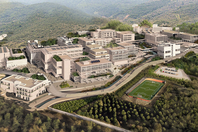
IZMIR UNIVERSITY OF ECONOMICS GÜZELBAHÇE CAMPUS

GLOBAL CAREER

CONTRIBUTION TO SCIENCE

VALUING PEOPLE

BENEFIT TO SOCIETY